Gradient descent algorithm in Machine learning

Machine Learning and Deep Learning commonly uses Gradient descent (GD) to find a local minimum/maximum of a given function. Gradient descent minimises a cost/loss function (e.g. in a linear regression).

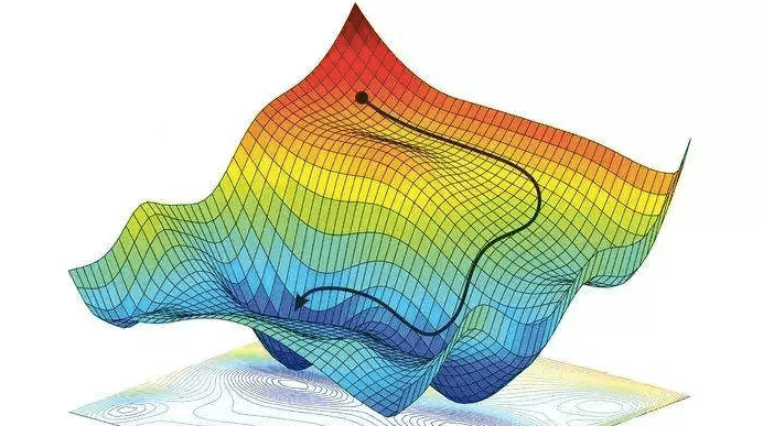
In mathematical terms, Gradient descent is a way to minimize an objective function J(θ) parameterized by a model’s parameters θ ∈ Rd by updating the parameters in the opposite direction of the gradient of the objective function ∇θJ(θ) w.r.t. to the parameters. The learning rate η determines the size of the steps we take to reach a (local) minimum. In other words, we follow the direction of the slope of the surface created by the objective function downhill until we reach a valley.

There are three variants of gradient descent, which differ in how much data we use to compute the gradient of the objective function. Choice of variant depends on accuracy and time taken to compute parameters.

Batch Gradient descent

A batch gradient descent, computes the gradient of the cost function w.r.t. to the parameters θ for the entire training dataset:

  θ = θ − η · ∇θJ(θ)

while True:
  grad_weights = calc_slope(loss_function, given_data, current_weights)
  current_weights
 += - step_size * grad_weights 

Batch gradient descent is guaranteed to converge to the global minimum for convex error surfaces and to a local minimum for non-convex surfaces.

• Needs whole dataset to perform just one update, so it can be slow
• If given_data doesn't fits to memory, computation can be expensive
• Not applicable for online dataset

Stochastic gradient descent

Stochastic gradient descent (SGD) in contrast performs a parameter update for each training example x (i) and label 

 y (i) : θ = θ − η · ∇θJ(θ; x (i) ; y (i) ) 

for i in range (nb_epochs):
    np.random.shuffle(given_data)
    for example in data :
        params_grad = calc_slope(loss_function , example , params )
        params = params - learning_rate * params_grad

Batch gradient descent performs redundant computations for large datasets, as it recomputes gradients for similar examples before each parameter update. SGD does away with this redundancy by performing one update at a time.

• Works with online dataset
• Performant effective
• Parameters can be fluctuating, it can help to jump to new and potentially better local minima.

Mini-batch gradient descent

Mini-batch gradient descent finally takes the best of both worlds and performs an update for every mini-batch of n training examples: 

θ = θ − η · ∇θJ(θ; x (i:i+n) ; y (i:i+n) )

In large-scale applications, the training data can have on order of millions of examples. Hence, it seems wasteful to compute the full loss function over the entire training set in order to perform only a single parameter update. A very common approach to addressing this challenge is to compute the gradient over batches of the training data.

while True:
  data_batch = sample_training_data(given_data, 256) 
  grad_weights = evaluate_gradient(loss_function, data_batch, weights)
  weights += - step_size * grad_weights

• Reduces the variance of the parameter updates, which can lead to more stable convergence;
• Can make use of highly optimized matrix optimisations

References

Image Creds https://easyai.tech/wp-content/uploads/2019/01/tiduxiajiang-1.png

https://arxiv.org/abs/1609.04747